X bar s chart excel
More than a bar chart this helps to represent data of comparison in more than one category. Under Chart Tools select the Design tab.

Control Chart Excel Template Inspirational Supply Chain View Free Excel Files For Six Sigma And Excel Templates Gantt Chart Templates Sign In Sheet Template
Add labels for the graphs X- and Y-axes.

. This describes the mechanics of axis label ordering. A clustered bar chart is generally known as a grouped bar chart. The stacked bar chart represents the given data directly but a 100 stacked bar chart represents the given data as the percentage of data that contributes to a total volume in a different category.
Right-click on the Bar representing Year 2014 and select Format. By selecting the formula bar rather than the values a formula will be displayed. This is a type of bar chart or column chart.
Go ahead based on your Microsoft Excels version. To do so click the A1 cell X-axis and type in a label then do the same for the B1 cell Y-axis. A preview of that chart type will be shown on the worksheet.
Display Settings - further define what the chart will look like. Figure D To finish the Excel chart delete the lines. 1 In Excel 2013s Format Axis pane expand the Labels on the Axis Options tab click the Label Position box.
This example illustrates how to create a clustered bar chart Create A Clustered Bar Chart A clustered bar chart represents data virtually in horizontal bars in series similar to clustered column charts. By default however Excels graphs show all data using the same type of bar or line. The R-chart generated by R also provides significant information for its interpretation just as the x-bar chart generated above.
In this quick tutorial well walk through how to add an Average Value line to a vertical bar chart by adding an aggregate statistic Average to a data set and changing a series chart type. How to Make a Clustered Stacked Bar Chart in Excel. Scatter charts are useful to compare at least two sets of values or pairs of data.
A clustered bar chart is a bar chart in excel Bar Chart In Excel Bar charts in excel are helpful in the representation of the single data on the horizontal bar with categories displayed on the Y-axis and values on the X-axis. Here is a generalized version that I wrote. In the Format Axis pane under Axis Options type 1 in the Maximum bound box so that out vertical line extends all the way to the top.
Esc key Remove the edits and a partial entry. In the same way engineers must take a special look to points beyond the control limits and to violating runs in order to identify and assign causes attributed to changes on the system that led the process to. Example 2 Clustered Bar Chart.
The advantage of a mirror bar chart is that it illustrates two data sets side by side and therefore makes it easy to make comparisons and spot any differences between them. You can even select 3D Clustered Bar Chart from the list. SpreadsheetWriteExcel tries to provide an interface to as many of Excels features as possible.
Scatter charts show relationships between sets. This tutorial uses Excel 2013. Highlight the data you want to cluster.
Enter key Edit the data in the current cell without moving the active highlighted cell to another. This would most likely be best as an XY Scatter chart with two series. R-chart example using qcc R package.
Where the bar chart draws the relation of two parameters this can consider the higher version of the bar chart. A blank column is inserted to the left of the selected column. There are 2 methods a simple version DisplaySimpleProgressBarStep that defaults to 20 Complete and a more generalized version DisplayProgressBarStep that takes a laundry list of optional arguments so that you can.
After adding the secondary horizontal axis delete the secondary vertical axis. A pie chart sometimes called a circle chart is a useful tool for displaying basic statistical data in the shape of a circle each section resembles a slice of pieUnlike in bar charts or line graphs you can only display a single data series in a pie chart and you cant use zero or negative values when creating oneA negative value will display as its positive equivalent and a. Set up the data firstI have the commission data for a sales team which has been separated into two sections.
You can change the color and style of your chart change the chart title as well as add or edit axis labels on both sides. Double-click the secondary vertical axis or right-click it and choose Format Axis from the context menu. 2D and 3D stacked bar.
Introduction to Grouped Bar Chart. A variety of bar charts are available and according to the data you want to represent the suitable one can be selected. For example a graph measuring the temperature over a weeks worth of days might have Days in A1 and Temperature in B1.
One using regular X values the other using normalized X values and both using the same Y values. Read more in simple steps. But 99 of the time a user expects the axis labels to go in the same order top to bottom as in the data source.
In frequentist statistics a confidence interval CI is a range of estimates for an unknown parameterA confidence interval is computed at a designated confidence level. As shown in the figure we must enter the data into. You can make many formatting changes to your chart should you wish to.
Right click the X axis in the chart and select the Format Axis from the right-clicking menu. The confidence level represents the long-run proportion of corresponding CIs that contain the true. For example you can get a Daily chart with 6 months of data from one year ago by entering an End Date from one year back.
To create a bar chart we need at least two independent and dependent variables. In this example I am going to use a stacked bar chart. While holding down the mouse the scale of the resized chart is shown to the left of the.
This chart tells the story of two series of data in a single bar. Price Box - when checked displays a Data View window as you mouse-over the chart showing OHLC for the bar and all indicator values for the given bar. How to Expand the Visibility of Formula Bar.
A vertical line appears in your Excel bar chart and you just need to add a few finishing touches to make it look right. Still they are visually complex. This will insert a Simple Clustered Bar Chart.
Updating the Data Set. In this chapter you will understand when each of the Scatter chart is useful. How to Convert a Pie Chart to a Bar of Pie Chart.
As a result there is a lot of documentation to accompany the interface and it can be difficult at first glance to see what it important and what is not. You will see a new menu item displayed in the main menu that says Chart Tools. In other Excel versions there may be some slight.
By default a bar chart in Excel is created using a set style with a title for the chart extrapolated from one of the column labels if available. These charts are easier to make. The chart resembles the reflection of a mirror hence the name mirror bar chart.
If more clustering is desired starting with the stacked bar chart with the blank row right-click on a bar and choose Format Data Series. The whole problem arises because Excel follows the same axis ordering scheme for bar chart category axes as for any other axis in any other chart. Right-click on the highlighted content and click Insert.
Click anywhere on the chart. The 95 confidence level is most common but other levels such as 90 or 99 are sometimes used. Shift F3 To get the dialog box to insert the functions.
If youve already created a Pie chart and now want to convert it to a Bar of pie chart instead here are the steps you can follow. Step 6 Double-click the chart type that suits your data. From the Insert Chart dialog box select the All Charts Bar Chart Clustered Bar Chart.
A 3D column chart may accommodate the data but not in a way that makes it at all intelligible. Read more which represents data virtually in horizontal bars in series. Now lets move to the advanced steps of editing this chart.
I needed an Excel VBA Progress Bar and found this link. You could leave the chart as is as a combo chart as shown in Figure D but lets remove the lines so its strictly a floating bar chart. The same can be activated using the shortcuts as.

Excel How To Create A Dual Axis Chart With Overlapping Bars And A Line Chart Visualisation Excel

Bar Graph Worksheets 5 Bars Single Unit Worksheet Bar Graphs Free Math Worksheets Teaching Math

Pin On Microsoft Office Tips

Python Plotting Charts In Excel Sheet Using Openpyxl Module Set 1 Geeksforgeeks Graphing Reading Writing Workbook
Creating Scrollable Data Ranges In Excel Excel Form Controls Scroll Bars Pakaccountants Com Excel Tutorials Excel Microsoft Excel Tutorial

The Nation S Favourite Takeaway Data Visualisation Food Charts Chartbuilder Data Data Visualization Chart Visualisation

Pin On Data Design

Sprint Burndown Chart Chart Project Management Templates Graphing

Dataviz Challenge 1 How To Make A Circle Chart In Excel Bubble Chart Data Visualization Chart

Flowchart Connector Lines In Excel Breezetree Excel Flow Chart Connector

Gantt Charts In Excel Tutorial From Jon Peltier Use Gantt Charts For Scheduling And Project Management Tasks Events Are Listed Alo Gantt Chart Chart Excel
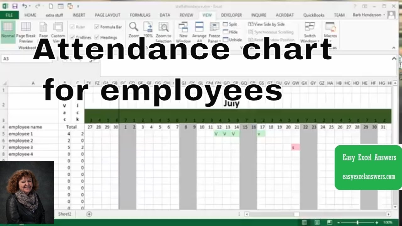
Make A Vacation Schedule Chart For Your Staff Page Layout Excel Chart

X Bar S Chart Formula And Calculation Average And Stdev Excel Formula Behaviour Chart Formula

Pin On Excel Tips Tricks Hacks Cheats

Swimmer Plots In Excel Peltier Tech Blog Excel Swimmer Chart

Excel Frequency Histogram And Relative Frequency Histogram Histogram Excel Templates Good Essay

Moving X Axis Labels At The Bottom Of The Chart Below Negative Values In Excel Pakaccountants Com Excel Excel Tutorials Chart